Outlier Detection Using K-means Clustering In Python
Introduction
In the previous article, we talked about how to use IQR method to find outliers in 1-dimensional data. To recap, outliers are data points that lie outside the overall pattern in a distribution. However, the definition of outliers can be defined by the users. In this article, we’ll look at how to use K-means clustering to find self-defined outliers in multi-dimensional data.
K-means clustering
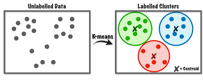
K-means clustering is an unsupervised distance-based machine learning algorithm that divides the data set into several non-overlapping clusters.
We won’t go through the detail of K-means clustering. Basically, we don’t have the label of data, so we want to divide data into several groups based on their characteristics. For example, we might want to group our customers based on their consuming habit.
Also, we want the inter-cluster distance (distance between each group) to be large, while the intra-cluster distance (distance between data points within a single cluster) to be small. By achieving this, the groups are more distinguishable, and the subjects within a single group are more alike.
One thing to note is that we need to specify the number of clusters (K) before training a model. In some cases, some data points are far from its own cluster, and we typically define them as outliers or anomalies.

Outlier detection
The interesting thing here is that we can define the outliers by ourselves. Typically, we consider a data point far from the centroid (center point) of its cluster an outlier/anomaly, and we can define what is a ‘far’ distance or how many data points should be outliers.
Let’s look at an example to understand the idea better. Say we collect the annual income and the age data of 100 customers, and we store the data in a data frame called customer. In specific, we want to separate them into several groups to depict their consuming habit.
1. Standardize the variables
The first thing we do is standardizing the variables to have mean as 0 and standard deviation as 1. The standardization is important since the variables have different ranges, which would have serious effect on the distance measure (i.e. Euclidean distance). In other words, the range of Income is much larger than that of Age, so the difference between ages would be ignored by K-means clustering algorithm.
ss = StandardScaler()
customer = pd.DataFrame(ss.fit_transform(customer), columns=['Income', 'Age'])
2. Data visualization — decide K
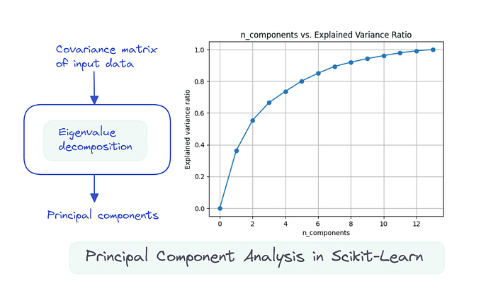
The second thing we do is visualizing the data through scatter plot in the hope of finding appropriate K. If the data set has more than 2 independent variables, principal component analysis (PCA) is required before visualization. However, we only have 2 variables here so we can directly make the plot.
plt.figure(figsize=(8,6))
plt.scatter(customer.Income, customer.Age)
plt.xlabel('Annual income')
plt.ylabel('Age')
plt.title('Scatter plot of Annual income vs. Age')
plt.show()
It’s obvious that the data can be roughly separated into 4 groups, so we can specify the K as 4 and train a K-means model.
⚡ We are lucky to have such distinguishable data set. Most of time the data is messy and we have to do cross validation to find the appropriate K.
3. Train and fit a K-means clustering model — set K as 4
km = KMeans(n_clusters=4)
model = km.fit(customer)
This step is quite straight-forward. We just feed all the variable we have to K-means clustering algorithm since we don’t have the target variable (i.e. the consuming habits of customers).
4. Cluster visualization
Now each data point is assigned to a cluster, we can fill the data points within a cluster with the same color. Also, we use black dots to mark the center of each cluster.
colors=["red","blue","green","orange"]# figure setting
plt.figure(figsize=(8,6))
for i in range(np.max(model.labels_)+1):
    plt.scatter(customer[model.labels_==i].Income, customer[model.labels_==i].Age, label=i, c=colors[i], alpha=0.5, s=40)
plt.scatter(model.cluster_centers_[:,0], model.cluster_centers_[:,1], label='Centers', c="black", s=100)
plt.title("K-Means Clustering of Customer Data",size=20)
plt.xlabel("Annual income")
plt.ylabel("Age")
plt.title('Scatter plot of Annual income vs. Age')
plt.legend()
plt.show()
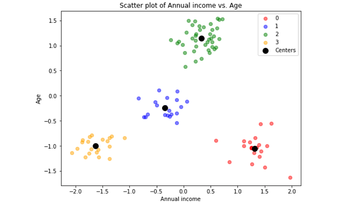
Here is our clustering. Generally speaking, the cluster goes as what we expected. Nevertheless, some data points seem to be far away from the center of its cluster (black dots), and we might classify these data points as outliers.
5. Outlier detection
Before we define what an outlier is, we need to calculate the distance of each data point from its center. To do this, we can create a new column label matching the clustering result. Then, we use distance_from_center function to compute the Euclidean distance and save the result in a new column called distance.
def distance_from_center(income, age, label):
    '''
    Calculate the Euclidean distance between a data point and the center of its cluster.:param float income: the standardized income of the data point
    :param float age: the standardized age of the data point
    :param int label: the label of the cluster
    :rtype: float
    :return: The resulting Euclidean distance
    '''
    center_income =  model.cluster_centers_[label,0]
    center_age =  model.cluster_centers_[label,1]
    distance = np.sqrt((income - center_income) ** 2 + (age - center_age) ** 2)
    return np.round(distance, 3)customer['label'] = model.labels_
customer['distance'] = distance_from_center(customer.Income, customer.Age, customer.label)
Now we can define our own outliers. Say we define the most distant 10 data points as outliers, we can extract them by sorting the data frame.
outliers_idx = list(customer.sort_values('distance', ascending=False).head(10).index)
outliers = customer[customer.index.isin(outliers_idx)]
print(outliers)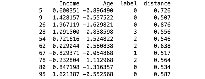
Voila! Here are our 10 outliers! They are defined as outliers since they are far away from the center, and we can further verify this through scatter plot.
# figure setting
plt.figure(figsize=(8,6))
for i in range(np.max(model.labels_)+1):
    plt.scatter(customer[model.labels_==i].Income, customer[model.labels_==i].Age, label=i, c=colors[i], alpha=0.5, s=40)
plt.scatter(outliers.Income, outliers.Age, c='aqua', s=100)
plt.scatter(model.cluster_centers_[:,0], model.cluster_centers_[:,1], label='Centers', c="black", s=100)
plt.title("K-Means Clustering of Customer Data",size=20)
plt.xlabel("Annual income")
plt.ylabel("Age")
plt.title('Scatter plot of Annual income vs. Age')
plt.legend()plt.show()
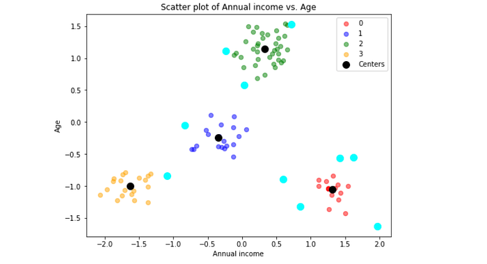
Indeed, the outliers (light blue points) are distant from the center. However, this is not the only way to define outliers. We can also define outliers as data points with distance larger than 0.8. Further, the outliers should NOT be removed immediately, they are instead worth-investigated. For instance, we might wonder why the characteristics of certain customers are different from their groups and we might surprisingly develop new customers!
💛💛💛 If you like this article, make sure to follow me! It really encourages me and motivates me to keep sharing. Thank you so much.
Coding
References